Heritability 201: Types of heritability and how we estimate it

In Heritability 101 we defined heritability as “the proportion of variation in a trait explained by inherited genetic variants.” In practice we’ll often rely on variations of this definition, in part because of the differences between this idealized concept of heritability and the reality of what we can actually estimate scientifically. In this post we’ll outline some different “flavors” of heritability, and the ways they can be estimated, with the end goal of explaining what form of heritability we’re reporting from the data of the UK Biobank.

The quick version:

Our UK Biobank analysis is estimating $h^2_g$, or SNP-heritability. This is only the proportion of variation in the trait that can be explained by additive effects of commonly-occurring genetic variants called SNPs (a single base change in a DNA sequence), so it’s almost always less than the total heritability $(H^2)$ that could be explained by all genetic factors.

We’re estimating $h^2_g$ using a method called LD score regression (LDSR); if the choice of method matters to you then you’ll probably appreciate the more technical post here.

 

Measuring variation

Before talking about the different flavors of heritability, it’s useful to define what we mean by “variation” when we say things like the “the proportion of variation in a trait explained by” something.

Here, when we say “variation”, we’re referring to the mathematical concept of “variance”. Variance is a common metric for measuring how much a trait differs between people in a group. Formally, it’s the average squared difference between a randomly selected person and the “average” person. For example, across all men and women in the UK Biobank the variance of height in inches is 13.3 (86.0 for height in centimeters), corresponding to a standard deviation of 3.7 inches (9.3 cm). The standard deviation is simply the square root of the variance.

Statisticians like talking about variance (as opposed to more intuitive measures like the range or the mean absolute deviation from average) because it has nice mathematical properties. Most notably, if you have an outcome that is the sum of effects from independent sources (like, say, genes and environment) the variance of the effects from each source add up to the variance of the outcome. Being able to break up the total variance of a trait into different pieces that add up this way is very useful when we want to start talking about the “proportion of variance explained by genetics”, as we will see below.

Lastly, talking about variance implicitly means we’re talking about a group or population of individuals. You can’t have an average difference between people with only one person. As we emphasize in Heritability 101, this means that whenever we talk about heritability we are talking about variation in some population of individuals, not about genetics determining some proportion of a trait in any given individual.

“Explaining” variance

It’s also worth clarifying the other half of the phrase “the proportion of variation in a trait explained by”, namely what we mean by “explained”. In this case, variance that is “explained” by genetics is variance that could be predicted based on genetic data if we had perfect information about the effects of all genetic variants (which, to be clear, we don’t actually have).

If you’ve ever heard the phrase “correlation is not causation”, that’s the issue we're referring to here and why we aren’t simply saying the proportion of variance caused by genetic effects. We are closer to causation since it’s fairly safe to assume that the heritable traits aren’t causing the genetic variants, since our genetics is fixed at conception (with the exception of acquired mutations such as those seen in cancer). It is possible, however, for genetic variants to be correlated with environmental factors that have a direct causal impact on the trait. That doesn’t mean the genetics aren’t important and informative for that trait, but it does mean we have to be careful about describing effects as causal, even in genetics. So as a precaution against making any premature statements about causality we focus on “explained” variance instead.

Broad-sense heritability

Our starting definition of heritability as “the proportion of variation in a trait explained by inherited genetic variants” refers to this most general version of heritability. Mathematically, we’d define the broad-sense heritability as:  $$H^2 = \frac{\sigma^2_G}{\sigma^2_P}$$  where $𝜎^2_G$ is the variance in the trait explained by genetics (G), and $𝜎^2_P$ is the total variance of the trait in the population.

We make three important observations about this definition. First, it’s entirely flexible about how specific genetic effects contribute to $𝜎^2_G$. The broad-sense $H^2$ doesn’t care whether $𝜎^2_G$ comes from a single Mendelian variant in just one gene, or the small additive effects from variants in 100 different genes, or complex interactions between every variant in the whole genome. We’ll see below that this is an important distinction between broad-sense $H^2$ and some of the other types of heritability.

Second, broad-sense $H^2$ is entirely flexible about how $𝜎^2_G$ relates to $𝜎^2_P$. We could choose to assume that the effects of genes and environment are independent and thus write:

$$H^2 = \frac{\sigma^2_G}{\sigma^2_G + \sigma^2_E}$$  but that assumption isn’t required. By simply writing the denominator as $𝜎^2_P$  we allow for the possibility that genetic and environmental factors are correlated or interact in some way. This is important since it highlights that the effect of environment on the trait isn’t simply the “remainder” after accounting for all the genetic effects, instead they can overlap and interact in complex ways.

Narrow-sense heritability 

In practice, the flexibility of broad-sense $H^2$  makes it very hard to estimate without making strong assumptions. Allowing for effects of all possible interactions of all possible genetic variants means having a functionally infinite space of possible effects. One useful way to simplify this is to think of the total variance explained by genetics as a combination of additive effects, dominant/recessive effects, and interaction effects between different variants. $$\sigma^2_G = \sigma^2_A + \sigma^2_D + \sigma^2_I$$

For a number of reasons, we might expect the variance explained by additive genetic effects $𝜎^2_A$ to be the largest and most immediately useful portion of the total $𝜎^2_G$ [1]. Focusing on just this additive genetic component leads us to the definition of the narrow-sense heritability $h^2$: $$h^2 = \frac{\sigma^2_A}{\sigma^2_P}$$

If there are no dominant/recessive or interaction effects (i.e. $𝜎^2_D = 𝜎^2_I = 0$) then the narrow-sense and broad-sense heritability are the same ($h^2 = H^2)$. Otherwise the narrow-sense heritability will be smaller ($h^2 < H^2$) since it excludes these other types of genetic effects.

Historically, most scientific discussion of the heritability of different traits has focused on $h^2$. One of the nice features of $h^2$ is that it implies a simple relationship between between how genetically related two people are and how similar the trait will be for those two people. We can use this relationship to estimate $h^2$ in twin and family studies.

In the simplest case, we can compare monozygotic twins (often called “identical” or MZ twins) to dizygotic (“fraternal” or DZ) twins. MZ twins shared all of their DNA [2], while DZ twins share half of their DNA on average. Twins also largely share the same environment regardless of whether they are MZ or DZ [3]. So to estimate $h^2$ we can observe how correlated a trait is between pairs of MZ twins and how correlated the trait is between DZ twins and see if those correlations are different. If the MZ twins pairs, with their higher genetic similarity, are more strongly correlated than the DZ twin pairs, that suggests that genetics explains some of the variance in the trait [4].

There has been decades of scientific research on the heritability of human traits using this general approach. Helpfully, a recent effort by Danielle Posthuma and colleagues pooled together much of this work into a single webpage where you can browse twin-based estimates of $h^2$ for a wide variety of traits. 

SNP-heritability

The above flavors of heritability have referred to “genetic effects” conceptually without requiring any consideration of specific genetic variants and their association with the trait. Now that advances in genetics [5] have made it possible to actually collect data on these specific variants, there’s the opportunity to evaluate how much each of these observed variants contribute to heritability.

In particular we can consider one type of genetic variant called a single nucleotide polymorphism (SNP), which is a change of a single base pair of DNA at a specific location in the genome. For example, some people may have an A at that location, while other people have a G. There are millions of these locations in the genome that commonly vary between different people, and much of the current research in human genetics is focused on understanding the effects of these variants [6].

So given a set “S” of SNPs that we’ve observed, how much of the variance in the trait can they explain? That leads us to define the SNP-heritability $h^2_g$, the proportion of variance explained by additive effects of the observed SNPs, which we could write as: $$h^2_g = \frac{\sigma^2_{SNPs \in S}}{\sigma^2_P}$$

If we compare this to the above definitions, it’s evident that $h^2_g ≦ h^2 ≦ H^2$ since $h^2_g$ is limited to additive effects from only a subset of genetic variants.

This definition of $h^2_g$ still hides the effects of individual SNPs though, so it’s useful to introduce an alternate version. If we call our trait y, and say each SNP $x_j$ has an additive effect $𝛽_j$ [7], then we can write $$y = \sum_{SNPs \in S} x_j \beta_j + \epsilon$$

where $\epsilon$ is a residual term for effects not explained by the sum of the SNP effects. Each $x_j$ here encodes the number of alternative alleles an individual has at polymorphic site j, either as 0/1/2 counts or as a centered and standardized transformation of those counts (both are equivalent for our purposes here). We can then define $h^2_g$ based on the variance of this sum of SNP effects compared to the total variance of the trait: $$h^2_g = \frac{var(\sum_{SNPs \in S} x_j \beta_j)}{var(y)}$$

It’s worth highlighting two key features of $h^2_g$. First, you might notice that we’ve defined $h^2_g$ based on some set of SNPs “S”. In practice, this set of SNPs is going to depend on (a) the SNP data that has been observed and (b) the method used for estimating $h^2_g$. This makes it tricky to compare values of $h^2_g$ between different methods and different studies [8], though in most cases it’s safe to at least assume it refers to commonly-occurring SNPs. Second, the variance explained by SNPs may or may not reflect the effects of those particular SNPs as opposed to the effects of other genetic variants the SNPs are correlated with. This is just an extension of our previous discussion above about the meaning of variance “explained”, but worth reiterating since it would be easy to misinterpret SNP-heritability as fully excluding the causal effects of other types of genetic variation.

There are a couple of different methods that have been developed for estimating $h^2_g$ from observed SNPs. In practice we don’t know the true $𝛽_j$ so we have to use other tricks. The first approach, known as GREML (Genomic relatedness matrix REstricted Maximum Likelihood; commonly implemented in GCTA), uses SNPs to estimate the genetic similarity between random individuals and compare that to their trait similarity. This is conceptually similar to the twin-based estimation described above, but uses the observed low-level genetic similarity in SNP data from individuals who aren’t directly related. You can read about the statistical details here with a more recent review here.

A second approach is called linkage disequilibrium (LD) score regression, implemented in ldsc. This is the method we are applying to the UK Biobank data set. LD score regression depends on the key observation that some SNPs are correlated with (i.e. in LD with) other genetic variants, so observing that SNP in turn “tags” information about the effects of other variants. The basic idea then is that if there are lots and lots of small genetic effects spread across the genome (i.e. the trait is “polygenic”), then the strength of the relationship between each individual SNP and the trait should be (on average) proportional to how much total genetic variation that SNP tags. Statistical details on the LD score regression method can be found here.

Variance explained by known SNP effects

All of the above flavors of heritability are defined based on the “true” variance explained by genetic variants. Although we noted above that we don’t know the true effects $𝛽_j$, we could estimate them from our observed SNP data and then use those estimated values to directly compute:   $$h^2_{PRS} = \frac{var(\sum_{SNPs \in S} x_j \hat{\beta_j})}{var(y)}$$

We refer to this version of heritability as $h^2_{PRS}$ since the sum with estimates $𝛽_j$ is often known as a polygenic risk score (PRS). As with $h^2_g$, it depends on the choice of a set S of SNPs. When this set is chosen to be only SNPs reaching genome-wide significance for evidence of association with the trait, this flavor of heritability is sometimes known as $h^2_{GWAS}$.

Estimating $h^2_{PRS}$ is valuable because it indicates how well we can predict the trait from the observed SNPs with our current estimates of $𝛽_j$. In comparison, $h^2_g$ indicates how well we could theoretically predict the trait from SNPs if we knew their true effect sizes. Inevitably $h^2_{PRS} ≦ h^2_g (≦ h^2 ≦ H^2)$ since uncertainty in our estimates of $𝛽_j$ reduces our prediction accuracy, but it’s a useful way to contextualize $h^2_g$ as the idealized maximum for $h^2_{PRS}$.

A note on liability vs. observed scale heritability

To some extent talking about components of the variance of a trait assumes the trait is continuous. For binary traits, such as whether or not someone is diagnosed with a disease, the use of variance as a convenient mathematical quantity becomes problematic.

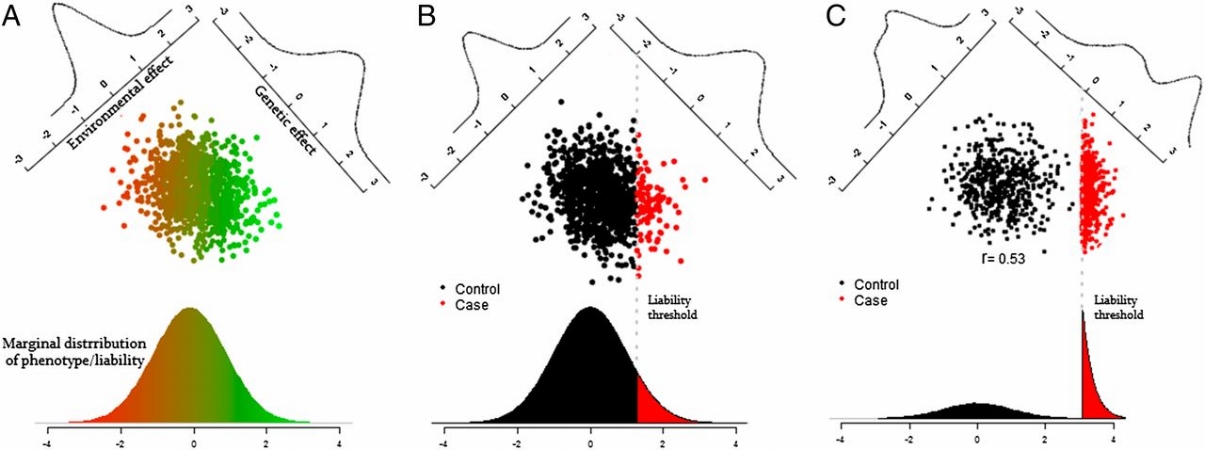
The conventional solution is to treat the binary trait as if it has an underlying continuous liability, as depicted above, and then quantify the heritability of that continuous liability. In other words estimate the genetic contribution to the continuous liability as shown in the left plot, based on observing the binary outcome of that liability as shown in the center plot. In some cases we may intentionally select more individuals who have the binary outcome, as shown in the right plot, in which case we have to further adjust the heritability calculations for how that ascertainment has changed the distribution of liability in our sampled individuals.

The mathematical details of that adjustment to get heritability estimates on the liability scale [9] aren’t critical, but it’s important to be aware that we’re having to make this additional adjustment for binary traits. This adjustment requires making assumptions about the prevalence of the trait in the population, which may or may not be safe in the UK Biobank data depending on the trait. As a result, the estimates of heritability for binary traits should be interpreted carefully, with an expectation that they are at a higher risk of statistical artifacts than than heritability estimates for continuous traits.

Summary

Hopefully we’ve provided some useful context when we say that in UK Biobank data set we’re estimating the SNP-heritability $h^2_g$ using LD score regression. Assuming our estimate is well calibrated (see Heritability 501 for lots more discussion of the technical limitations), we can anticipate that this $h^2_g$ is less than the full contribution of genetics to each trait $(h^2_g ≦ h^2 ≦ H^2)$ and more than our current ability to predict each trait from the genetic data $(h^2_{PRS} ≦ h^2_g)$. There will be additional uncertainty in these estimates for binary traits.

Correction

4/23/2019: This page was updated to include the sentence "Each x_j here encodes the number of alternative alleles an individual has at polymorphic site j, either as 0/1/2 counts or as a centered and standardized transformation of those counts (both are equivalent for our purposes here)" for clarity.

Footnotes

[1]

Except in extreme edge cases, $𝜎^2_A$ will capture a portion of the variance explained by genetic variants acting through dominant, recessive, or epistatic effects. Additive effects are also well-behaved statistically, making estimation of additive effects easier than the other components of $𝜎^2_G$. Estimates that have included dominant/recessive and/or interaction effects fairly consistently identify $𝜎^2_A$ as the largest component. As a result, most current work on common genetic effects focuses on this additive component. It probably misses some things, but it’s a useful simplification.

[2]

De novo mutations, mosaicism, etc potentially prevent the whole-genome sequences of monozygotic twins from being truly identical, but it’s close enough for most purposes here.

[3]

Again we’re simplifying, but for twins raised together we can generally expect them to at least share the same parents, childhood home, schools, neighborhood, etc. There’s plenty of research on this “common environment” aspect of twin modelling, for the sake of explanation we’re focusing on the idealized version here.

[4]

Specifically, given trait correlations $r_{MZ}$ and $r_{DZ}$ between the MZ twin pairs and DZ twin pairs, respectively, the estimate of $h^2$ is $2*(r_{MZ}-r_{DZ})$.

[5]

The Human Genome Project to provide a map of the human genome, the HapMap Project identify the structure of genetic variation in the human population, advances in genotyping and sequencing technology to allow robust and efficient measurement of genetic variants, to name a few.

[6]

This is mostly because they are cheaper and easier to observe. That certainly doesn’t mean there isn’t research on other types of genetic variation though. Insertions, deletions, duplications, and other genetic modifications are all also areas of active research.

[7]

These are $𝛽_j$ from the best linear predictor of the trait from the set of SNPs S. Importantly, this means these $𝛽_j$ are not the causal effects of each SNP, nor are they the marginal GWAS $𝛽_j$. Instead, they’re a projection of the causal effects of all genetic variants to the chosen “universe” of SNPs. As a result the $𝛽_j$ still exist as population parameters for that projection, but are entirely dependent on the chosen set of SNPs.

[8]

As an aside for those familiar with LD score regression, this is part of benefit of standardizing analysis to use the common HapMap3 SNPs and pre-computed reference LD scores. It doesn’t fully eliminate the differences between analyses, but it does keep them closer so there’s room for at least some intuition about what constitutes a “large” or “small” ldsc $h^2_g$.

[9]

Mathematically, the conversion between the heritability of the observed binary trait and the more interpretable heritability of the continuous liability is computed as: $$h^2_{liability} = h^2_{observed} \frac{K(1-K)}{\varphi(\Phi^{-1}[K])^2} \frac{K(1-K)}{P(1-P)}$$

where $K$ is the frequency of the binary trait in the population, $P$ is the frequency of the binary trait in the observed sample, and the denominator of the first fraction is the squared probability density function evaluated at the $K$ quantile of the inverse cumulative density function of the standard normal distribution. Derivation of this conversion in the genetics context can be found here, but note that does not perfectly resolve the issue of ascertained binary traits.

Authored by Raymond Walters with contributions from Claire Churchhouse and Rosy Hosking